Vision in Degraded Visibility Conditions
I have been working on vision in degraded visibility conditions (fog, rain, snow, and nighttime) for a long time. Over the years I have made progress on many facets the problem, and many things in the field of vision has also changed along the way. I will outline some interesting aspects in this post.
Introduction to Atmospheric Scattering
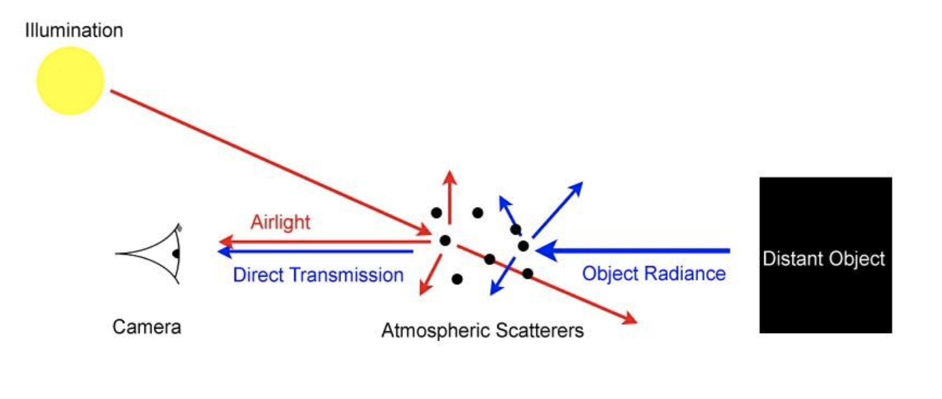
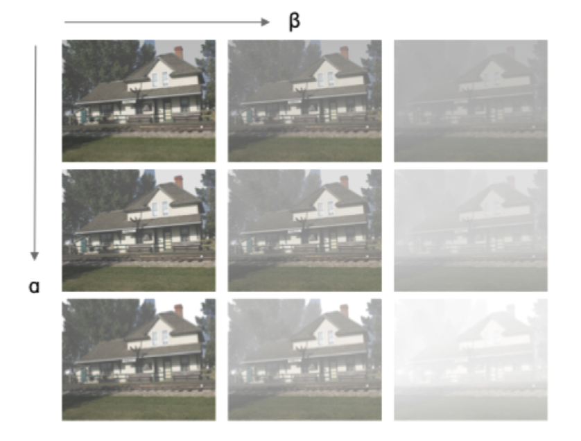
To motivate the problem, consider the scenario where you are given a single foggy RGB image and you want to obtain the defogged image. Before we delve into the details, let’s first understand the physics of fog. Fog is a weather phenomenon that occurs when the air is saturated with water vapor. The water droplets in the air scatter light (a phenomenon known as Mie scattering), which reduces the contrast and visibility of objects in the scene. Let \(L\) be the luminance of an object under monochromatic light, \(L_0\) the luminance at zero distance, \(\beta\) Mie scattering parameter, and \(\alpha\) background luminance (airlight). Both Koschmieder (1924) [1] and Duntley (1948) [2] showed the scattering of light is modeled by the following equation (Atmospheric Scattering Model):
\[L = L_0 e^{-\beta d} + \alpha (1 - e^{-\beta d})\]where \(d\) is the distance between the observer and the object. This model is applicable to visibility degredation through a scattering medium in general, and not limited to fog.
Humans are trichromatic and have cones for short, medium, and long wavelengths that correspond to our perception of blue, green, and red primary colors (1931 CIE color matching). The luminance of channel \(y\) is computed by integrated the respective color matching function \(y(\lambda)\) against the irradiance, \(E\), over all wavelengths.
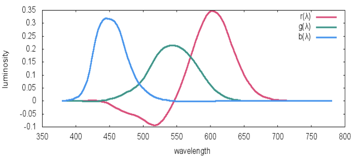
Without scattering, the luminance of each channel is given by
\[L_{y} = \int_{0}^{\infty} y(\lambda) E(\lambda) d\lambda\]Mie scattering is independent of wavelengths, that is with scattering, the luminance of each channel is given by the Atmospheric Scattering Model as
\[L_{y} = \int_{0}^{\infty} y(\lambda) \left[ E(\lambda) e^{-\beta d} + \alpha (1 - e^{-\beta d}) \right] d\lambda\]As the color matching functions are normalized to integrate to the same constant, and the transformation from CIE RGB to standard RGB colorspace is linear, for each of the RGB channels of the image we have
\[I(x) = J(x) t(x) + \alpha(1 - t(x))\]where \(I(x)\) is the observed luminance at pixel \(x\), \(J(x)\) is the scene luminance, \(t(x) = e^{-\beta d(x)}\) is the transmission map, \(d(x)\) the depth map, and we absorb the normalization constant into \(\alpha\). With some algebra, we can see to estimate the scene radiance \(J(x)\) we need to estimate the transmission map \(t(x)\).
Two early works, DehazeNet [3] and Dark Channel Prior [4], respectively estimated the transmission map directly in an end-to-end manner using a ConvNet and using the Dark Channel Prior. Once we have the transmission map, as in DehazeNet, \(\alpha\) can be estimated as
\[\alpha = \max_{y, x \in t(x) < t_0} I(x)\]where \(t_0\) is a tunable parameter.
Visibility Distance Estimation
While at Nvidia Self Driving, I worked on operational domain verification for autonomous vehicles. One of the tasks was to determine the meteorological visibility distance, which influenced the decisions made by the perception stack. We can rearrange the Atmospheric scattering model as follows
\[\frac{L - \alpha}{\alpha} = \left( \frac{L_{0} - \alpha}{\alpha} \right)e^{-\beta d}\]or equivalently
\[C = C_{0}e^{-\beta d}\]where \(C\) is defined as the visual contrast. The meteorological visibility distance is defined as the distance at which the visual contrast is reduced to a certain threshold, usually 0.05 of a black object (\(L_{0} = 0\)), which is approximately
\[d_{m} = -\frac{\ln(0.05)}{\beta}\]It is important to note visibility distance degredation is a global effect. This means local effects by lamppost glare, puddle reflections, vehicle spray do not contribute to the visibility distance. This does not mean we do not consider them; on the contrary, our model must learn how to recongize and ignore local effects. The team decided to train a CNN to regress visibility distance from synthetic data, as real images in degraded conditions were sparse due to collection bias.
If the only condition considered was fog, the solution would be straightforwards. In the real world, however, degraded visibility is usually observed with other weather conditions such as rain, sleet, or snow, as shown below

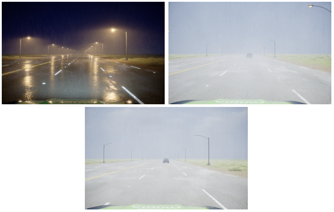
The team decided to generate data using DriveSim, Nvidia’s simulation engine, with global effects e.g. fog, rain, snow, sleet, or nighttime as well as local effects. Some examples of global and local effects at a fixed visibility degredation are shown below
To get the ground truth visibility from global effect parameters, we setup an interface with simple track scene with an black object. The interface would binary search for where the user can detect the object
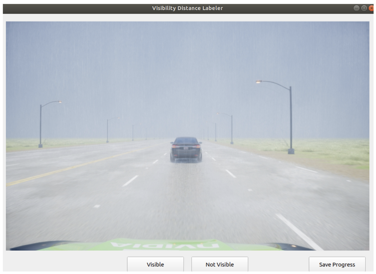
One issue however, was there is a large sim2real gap. Forunately, other projects had shown mixing real data with DriveSim data resulted the model generalizing well to real world data features. We decided to mix the DriveSim data with real visibility degraded data generated using the Atmospheric Scattering Model, estimating the depth maps via monocular depth estimation.
We show two examples of real foggy images collected from real life and a visibility degraded image generated from a real clear image below

The atmospheric model is quite powerful and can produce varying levels of degredation

Generated data can also be fed into a general data augmentation engine to produce different scenarios such as sand and dust storms

Verification with real data collected by test drives produced approximately reasonable results. In practice, the regressed visibility distance is classified into bins, and the car correspondingly switches autonomy levels based on the designated visibility bin.
In the Generative Model Era
The advent of generative diffusion processes opened up new avenues to the data augmentation aspect of the problem, specifically domain translation for autonomous vehicle dataset augmentation. Given a biased dataset of images collected under good driving conditions, can we construct foggy, rainy, snowy, and nighttime counterparts for each image, preserving structure and semantics but changing weather? Previous approaches such as CycleGAN and MUNIT have touched on this problem, but diffusion models provide an unprecented level of realism and control over the generated images.
I constructed a language model-based augmentation agent that performs rejection sampling of InstructPix2Pix [5]. Given an input image, the language model would propose edits that InstructPix2Pix carried out. InstructPix2Pix often fails to generate edits or corrupts the image— edited images below an LPIPs threshold are removed. The agent then proceeds recursively to the accepted edits. Optionally as a final step, the depth map of the input image is estimated and visibility degradation is applied using an atmospheric scattering model. The pipeline is illustrated below
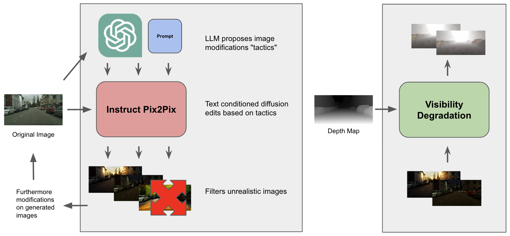
Here are some results of the agent, which is able to support a diverse array of quality edits far beyond what previous methods could achieve
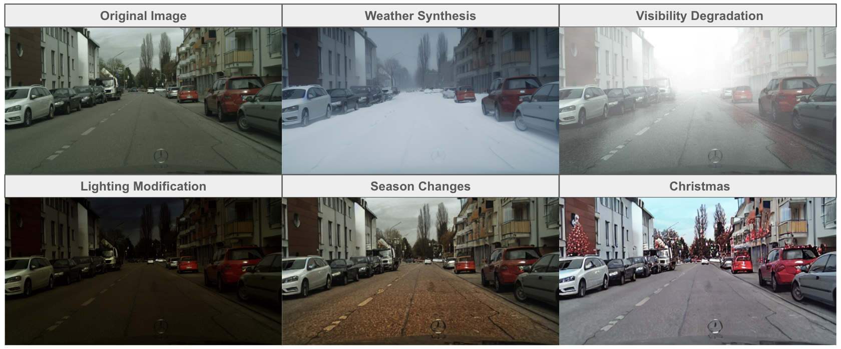
In general, the performance is decent but there are several issues with InstructPix2Pix:
- high corruption rate
- edit quality dependent on finetuning data
- does not support compositional domain translation e.g. a clear image is transformed to have a hybrid of weather conditions
where the last point is particularly important.
This led me to an alternative method: Schrodinger Bridge-based methods [6], [7], which are well grounded in theory and result in minimal corruption. They only rely on the diffusion model \(p_{\phi}(x)\) accurately modeling the source and target domain image distributions, compared to being finetuned on edits. In the case of [7] are defined as the diffusion model image distribution conditioned on keywords describing the source and target domains \(p_{\phi}(x, y_{\text{src}})\), \(p_{\phi}(x, y_{\text{tgt}})\). Given this setup, [7] provides a translation gradient to optimize the image \(x\) from the source to the target distribution
\[\nabla_x \mathcal{L}(x) \propto \mathbb{E}_{t, \epsilon}\left[ \epsilon_{\phi}(x_t, y_{\text{src}}, t) - \epsilon_{\phi}(x_t, y_{\text{tgt}}, t) \right]\]where \(x_t\) denotes the noised image and \(\epsilon\) denotes the learned score function for \(p_{\phi}(x)\). Below are some videos of domain translation in action for snow, nighttime, and rain. The edits are more realistic than InstructPix2Pix since Schrodinger Bridge-based methods are based on a notion of optimal transport between the conditional diffusion distributions.
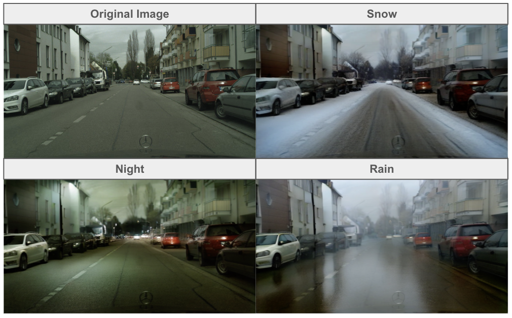
Simply changing the target domain’s text conditioning is not stable nor controllable. We found that simply following a linear combination of translation gradients between well defined domains can achieve compositional domain translation. The weights, however, may not be proportionally to the desired influence of the domain. As an example, suppose we are translating to both domains A and B. The translation gradient for domain A may need to be weighted higher than the translation gradient for domain B for the final image to have A and B equally present. We propose to translate the image to domains A and B separately. Then, we dynamically adjust the weights during compositional domain translation optimization using an image similarity model such as CLIP by comparing the similarity of the currently optimized image to the separately translated images. Instead of weight adjustment, assuming there is a large number of optimization steps, each step we can step towards one domain, adjusting the target as needed. Below we show some examples of interpolations between night and snow with different weights.

Schrodinger Bridge-based Methods
The theory behind Schrodinger Bridge-based methods is quite rich. Let \(\Omega = \mathbb{C}([0, 1], \mathbb{R}^n)\) denote the space of continuous paths over \([0, 1]\). Given \(W\), a reference probability measure on \(\Omega\), the Schrodinger Bridge Problem (SBP) seeks to find a measure \(P_{SBP}\) such that
\[P_{SBP} = \arg\min_{P} D_{KL}(P||W)\]for \(P \in D(p_0, p_1)\), where \(D\) denotes the collection of measures over \(\mathbb{C}\) with marginals \(p_0\) and \(p_1\).
SBP has connections to diffusion processes. When \(W\) results from the forward SDE of the variance exploding (VE) score generative model (SGM) that models \(p_{\text{data}}\) and results in \(p_{\text{prior}}\), SBP can be shown to produce solutions to an entropy-regularized Monge-Kantorovich (distribution mass) optimal transport problem between \(p_0\) and \(p_1\) [8]. In fact this shows that SGM themselves are solutions to entropy-regularized optimal transport with 0 KL divergence since we can set \(p_0 = p_{\text{data}}\) and \(p_1 = p_{\text{prior}}\). Note any VP SDE can be reparmetrized as a VE SDE.
To see this more clearly, note we can write the VE SDE forward and reverse processes as
\[\begin{align*} d\mathbf{x} &= \mathbf{f}(\mathbf{x}, t) \, dt + g(t) \, d\mathbf{w}, \\ d\mathbf{x} &= \left[\mathbf{f}(\mathbf{x}, t) - g(t)^2 \nabla_{\mathbf{x}} \log p_t(\mathbf{x}) \right] \, dt + g(t) \, d\mathbf{w} \end{align*}\]and SBP solution has forward and reverse processes of the form
\[\begin{align*} d\mathbf{x} &= \left[\mathbf{f}(\mathbf{x}, t) + g(t)^2 \nabla_{\mathbf{x}} \log \Phi_t(\mathbf{x}) \right] \, dt + g(t) \, d\mathbf{w}, \\ d\mathbf{x} &= \left[\mathbf{f}(\mathbf{x}, t) - g(t)^2 \nabla_{\mathbf{x}} \log \hat{\Phi}_t(\mathbf{x}) \right] \, dt + g(t) \, d\mathbf{w} \end{align*}\]where \(\mathbf{f}\) and \(g\) refer to the drift and diffusion terms in the VE SDE and has marginals \(p_t(\mathbf{x}) = \Phi_t(\mathbf{x})\hat{\Phi}_t(\mathbf{x})\) where \(\Phi_t(\mathbf{x})\) and \(\hat{\Phi}_t(\mathbf{x})\) are called Schrodinger factors the solution to certain PDEs involving \(\mathbf{f}\) and \(g\) and the boundary conditions \(p_0\) and \(p_1\) [9].
Let \(\mathbf{z}_t = g(t)\nabla_{\mathbf{x}}\log \Phi_t(\mathbf{x})\) and \(\hat{\mathbf{z}}_t = g(t)\nabla_{\mathbf{x}}\log \hat{\Phi}_t(\mathbf{x})\). Wen \(p_0 = p_{\text{data}}\) and \(p_1 = p_{\text{prior}}\), the Schrodinger factors are
\[(\mathbf{z}_t, \hat{\mathbf{z}}_t) = (0, g(t)\nabla_{\mathbf{x}} \log p_t(\mathbf{x}))\]which is exactly the SGM [9]. Each SBP SDE also has a corresponding ODE is a solution to the SBP and has the same marginals \(p_t\) [9]. Thus it also satisfies the optimal transport criteria.
\[d\mathbf{x} = \left[ \mathbf{f}(\mathbf{x}, t) + g(t)\mathbf{\mathbf{z}_t} - \frac{1}{2}g(t)\left( {\mathbf{z}_t + \hat{\mathbf{z}}_t} \right) \right]dt\]Substituting \((\mathbf{z}_t, \hat{\mathbf{z}}_t)\) from above, we get the probabability flow ODE for the SGM
\[d\mathbf{x} = \left[ \mathbf{f}(\mathbf{x}, t) - \frac{1}{2}g(t)^2\nabla_{\mathbf{x}}\log p_t(\mathbf{x}) \right]dt\]which has the same marginals as the VE SDE and is equivalent to a DDIM. Dual Diffusion Implicit Bridges (DDIB) [6] concatenates two DDIMs for unpaired image-to-image translation, which forms image to latent to image concatenation of optimal transport. This empirically works well. Since DDIMs are deterministic and reversible, DDIB guaruntee cycle consistency up to ODE discretization error.
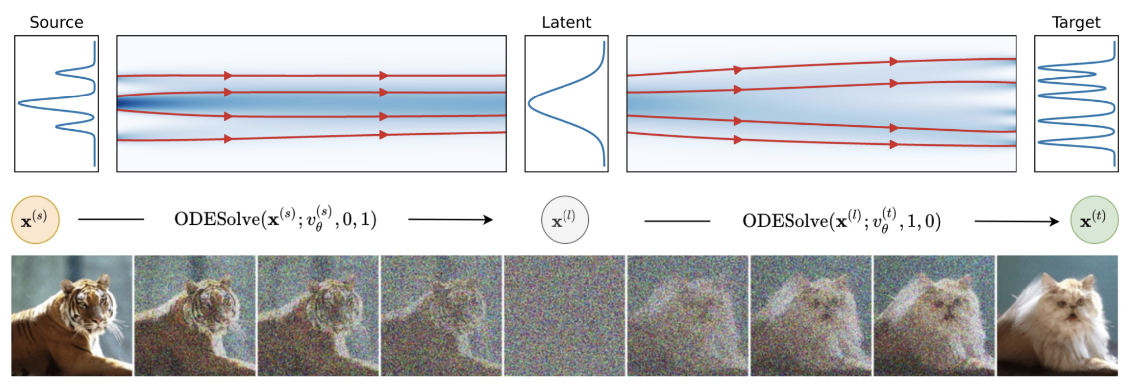
Suppose our distributions are text conditioned distributions \(p(\mathbf{x}\vert\mathbf{y})\) with score \(\epsilon(\mathbf{x}_t, \mathbf{y}, t)\). The DDIB translation is expressed as
\[\epsilon_{\text{SBP}}^* \cong \text{ODESolve}(\mathbf{x}_{\text{src}}, \mathbf{x}_T, p(\mathbf{x}\vert\mathbf{y}_{\text{src}})) \rightarrow \text{ODESolve}(\mathbf{x}_T, \mathbf{x}_{\text{tgt}}, p(\mathbf{x}\vert\mathbf{y}_{\text{tgt}}))\]One issue with DDIBs is they are slow as \(p_1\) must be the (DDIM reparametrized) prior distribution for the VE SDE i.e. fixed variance Gaussian, which means there are two full DDIM evaluations per translation. Instead, [7] proposes a one step linear approximation to DDIB as the difference of scores
\[\epsilon_{\text{SBP}} \cong \epsilon(\mathbf{x}_t, \mathbf{y}_{\text{tgt}}, t) - \epsilon(\mathbf{x}_t, \mathbf{y}_{\text{src}}, t)\]The figure below shows the linear approximation compared to full DDIB.
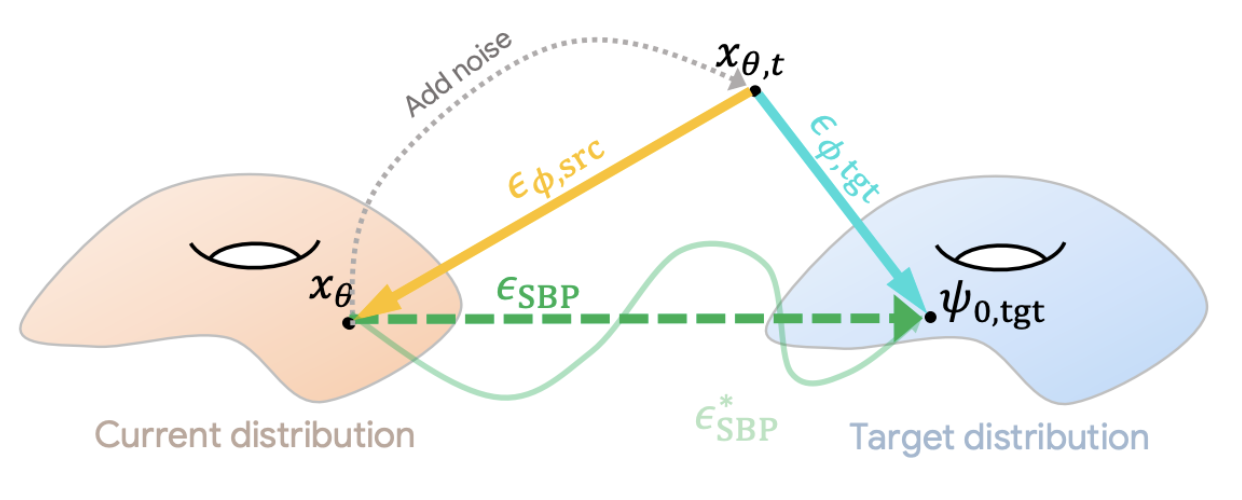
In practice, we take the translation gradient as proportional to
\[\mathbb{E}_{t, \epsilon}\left[ \epsilon_{\phi}(x_t, y_{\text{src}}, t) - \epsilon_{\phi}(x_t, y_{\text{tgt}}, t) \right]\]which is the gradient we saw above. This gradient can be applied less often than the number of UNet evaluations in DDIB and also enables compositional domain translation as shown above.
And so far that’s it. Thanks for reading and stay tuned for more updates on vision in degraded visibility conditions!
References
[1] Koschmieder, H., Theorie der horizontalen Sichtweite. Beitr. Phys. Atmos. 12, 33-58, 1906
[2] Duntley, S. Q., The visibility of distant objects. J Opt Soc Am., 1948
[3] DehazeNet: An End-to-End System for Single Image Haze Removal, 2016
[4] Single Image Haze Removal Using Dark Channel Prior, 2009
[5] InstructPix2Pix: Learning to Follow Image Editing Instructions, 2022
[6] Dual Diffusion Implicit Bridges for Image-to-Image Translation, 2023
[7] Rethinking Score Distillation as a Bridge Between Image Distributions, 2024
[8] Diffusion Schrödinger Bridge with Applications to Score-Based Generative Modeling, 2021
[9] Likelihood Training of Schrödinger Bridge using Forward-Backward SDEs Theory, 2022